EC 270 - 2026-09-17 - Lecture 03
EC 270 - Lecture 03 - 2026-09-17
Week 2 · 11:30-12:39 · 69 min · Full transcript · Flashcards
Overview
This lecture finished Chapter 2 with one last budget constraint case, a good with a negative price. It then covered all of Chapter 3: Preferences. Chapter 2 told us which bundles a consumer "can afford", and Chapter 3 starts to define which bundle is "best". McLeod built the language of preferences, added the axioms that keep preferences consistent, drew them as indifference curves, and finished with "well-behaved" preferences and the marginal rate of substitution (the slope of an indifference curve).
Negative prices
This is the last Chapter 2 example. It picks up right after Tuesday's non-linear (quantity-discount) pricing case.
A good with a negative price
A negative price means you get paid for every unit you consume. McLeod's example is commodity 1 as "stinky garbage": you don't want it, but someone will pay you to take it.
Why: When
where
Commodity 1 is stinky garbage with
-- put the prices and income into the budget constraint -- move the garbage term to the right: spending on good 2 equals income plus $2 per unit of garbage -- the slope is positive, so the line slopes upward -- vertical intercept: consume no garbage and spend all $10 on good 2 -- the horizontal intercept is at a negative quantity, outside the quadrant we draw
Answer: The budget line starts at
left=0; right=10; bottom=0; top=30
---
y=10+2x|x>0
(0,10)|label:Vertical intercept
x is units of stinky garbage (
When McLeod asked for the slope of the budget line, a student answered "negative P2 over P1". McLeod's reply was "Oh, so close." The slope is
Preferences and choice
Chapter 2 defined what the consumer "can afford". Chapters 3 and 4 work together to define what is "best": Chapter 3 builds the language of preferences, and Chapter 4 turns it into a working model.
The behavioural postulate
The assumption is that a decision maker always chooses their most preferred alternative from the set of alternatives available to them. So to model choice, we have to model preferences.
Why: It's a fancy way of saying that when you look at your options, you can pick the one you like best. McLeod's example: in a grocery store you can pick the item you like more than everything else, like a T-bone steak.
Three preference relations
A consumer compares two bundles,
- Strict preference,
: the consumer wants X rather than Y. The symbol looks like a greater-than sign with a squiggle. - Indifference,
: X and Y are equally good, and the consumer would be just as satisfied with either. The symbol is a tilde. - Weak preference,
: X is at least as good as Y, and maybe better. Think of it as a greater-than-or-equal-to sign.
Preferences are ordinal
All three relations are ordinal. They only rank bundles (first, second, tied). They never say how much more one bundle is liked.
Why: None of these statements says "I like X twice as much as I like Y." Preferences are about rank order, not size. McLeod said the course will come back to why only rankings matter.
How the relations fit together
The three relations depend on each other. If a consumer is logically consistent, combining statements must lead to a logical conclusion:
- Weakly preferring X to Y and also weakly preferring Y to X means the consumer is indifferent.
- Weakly preferring X to Y but not weakly preferring Y to X means X is strictly preferred.
where X and Y are two consumption bundles.
Axioms of consistent preferences
The relationships above don't go far enough on their own. These three axioms (assumptions) make sure preferences are logically and rationally consistent.
Completeness
For any two bundles, the consumer can always make one of these statements: X is weakly preferred to Y, Y is weakly preferred to X, or the consumer is indifferent between them. The consumer doesn't have to state a strict preference. They just can't be unable to compare.
where X and Y are any two bundles.
Reflexivity
Any bundle is at least as good as itself.
Why: It seems obvious once it's written down. It rules out nonsense like strictly preferring X to X.
where X is any bundle.
Transitivity
If X is at least as good as Y, and Y is at least as good as Z, then X is at least as good as Z.
Why: It rules out "something weird", like the consumer then turning around and strictly preferring Z to X. It is also the axiom behind the proof that indifference curves can't cross.
where X, Y and Z are three bundles.
McLeod called transitivity "probably... the most important of the three" axioms, and said the course would come back to why the axioms matter.
Indifference curves
This is the graphical version of the indifference statement, drawn in the same
Indifference curves
Pick a reference bundle
Why: If the consumer is indifferent among a few bundles, there are probably many more bundles they feel the same about. Drawing a line through all of them shows the whole set. The name is just a convention. An indifference "curve" is not always curved (it can be a straight line), so think of it as an indifference "set".
Ranking bundles with indifference curves
Bundles above the indifference curve through
Why: Consumers generally like more stuff. Z has more of both commodities than a bundle on
There is an infinite number of indifference curves, because every bundle in the quadrant has one passing through it. If you drew them all, the graph would be "a solid mass of dark purple".
Weakly and strictly preferred sets
- Weakly preferred set: all bundles on or above
. These are the bundles the consumer likes just as much as or more. It includes the curve itself.
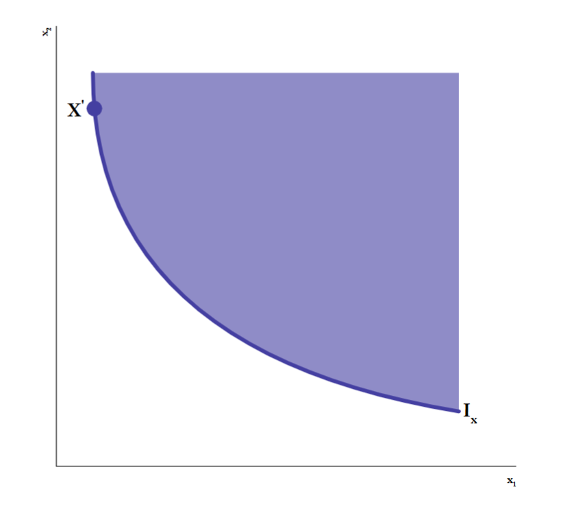
- Strictly preferred set: all bundles strictly above
. These are the bundles the consumer likes more than . It does not include the curve.
Indifference curves cannot cross
Indifference curves for different levels of preference can never intersect. McLeod proved this by contradiction: assume they do cross, and show that it breaks transitivity.
Why: Suppose curve
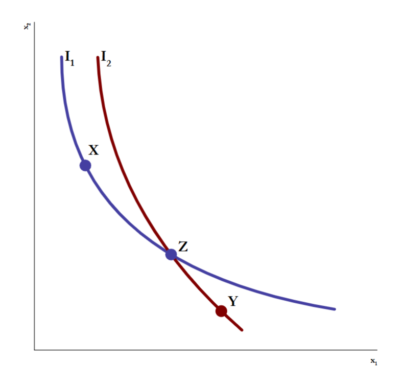
McLeod stated this as a claim and proved it in class: "indifference curves will never intersect... given our assumption of transitivity." Be ready to reproduce the contradiction argument.
Shapes of indifference curves
The shape of an indifference curve depends on whether each commodity is liked or not, and on the consumer's underlying preferences.
Goods, bads and neutrals
McLeod pointed out that "commodity" is the neutral word. Calling something a "good" already makes a judgment that more of it is better.
- Good: more of it is always preferred. If both commodities are goods, indifference curves slope downward, and "better" is up and to the right.
- Bad: less of it is always preferred, like stinky garbage. With one good on the horizontal axis and one bad on the vertical axis, indifference curves slope upward. Moving right makes you better off, and moving up and to the left makes you worse off.
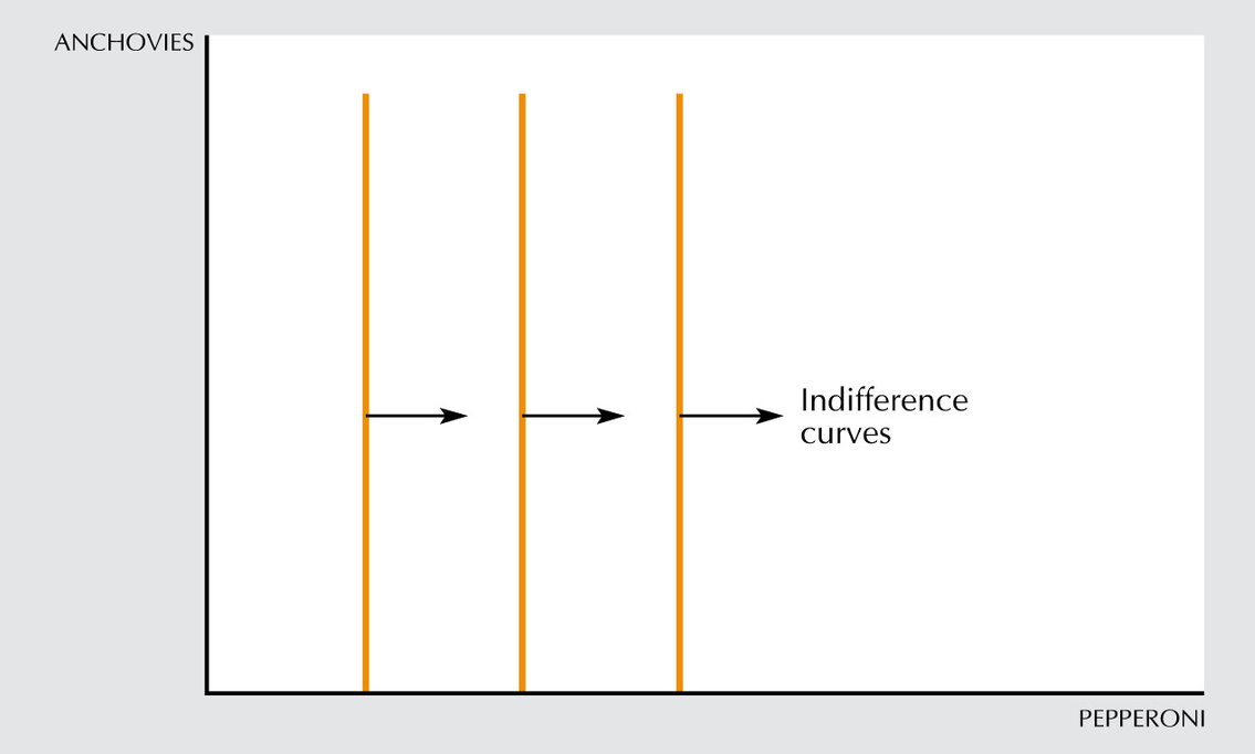
- Neutral: the consumer doesn't care how much of it they have. With the good on the horizontal axis and the neutral on the vertical axis, indifference curves are vertical. If the neutral is on the horizontal axis instead, they are horizontal.
- Example: If a consumer really likes pepperoni but is neutral about anchovies, then adding extra anchovies won't move the consumer to a different indifference curve and thus it only matters as to how much pepperoni there is (this example is from the textbook, not from class):
Perfect substitutes
The consumer sees the two commodities as completely interchangeable - the consumer will substitute one good for the other at a constant rate. Only the total amount in the bundle decides the ranking. Indifference curves are straight lines with a constant slope of
Why: The consumer is always willing to swap one unit of one commodity for one unit of the other, so the rate of exchange never changes.
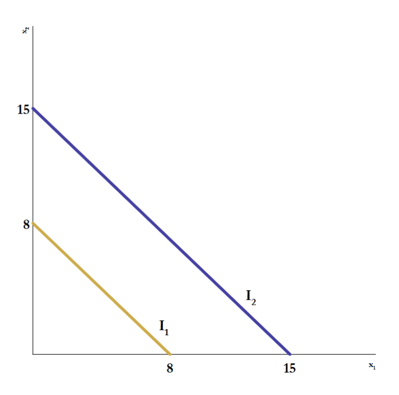
On
and -- the bundles and have the same total, so both are on -- the slope between the two points -- any bundle totalling 15 has more in total than any bundle on
Answer: Every bundle on
left=0; right=16; bottom=0; top=16
---
y=8-x
y=15-x
x is units of commodity 1 and y is units of commodity 2. The lower line is
Perfect complements
The consumer always consumes the two commodities together in a fixed proportion, here one to one, so they come in "pairs". Only the number of pairs decides the ranking. Indifference curves are L-shaped, with the corner where
Why: Adding more of only one commodity doesn't make a new pair, so the consumer is no better off. You only reach a higher curve when both go up together in the fixed proportion.
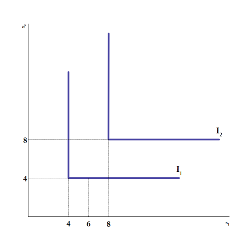
Compare the bundles
gives 4 pairs -- this is the corner of still gives 4 pairs -- the 2 extra units of good 1 have no partner, so this bundle is on the flat arm of still gives 4 pairs -- the 2 extra units of good 2 have no partner, so this bundle is on the vertical arm of gives 8 pairs -- both goods went up together, so this bundle reaches
Answer: The first three bundles are equally good, and
left=0; right=12; bottom=0; top=12
---
x=4|y>4
y=4|x>4
x=8|y>8
y=8|x>8
(4,4)|label:I1 corner
(8,8)|label:I2 corner
x is units of commodity 1 and y is units of commodity 2.
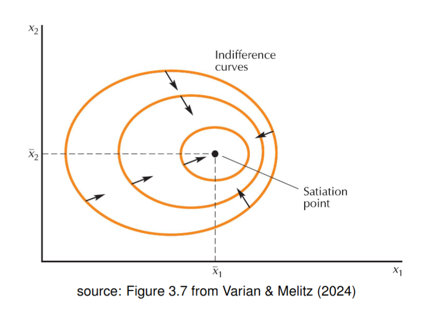
Satiation
The satiation (bliss) point
Why: Think of the usual downward-sloping curves as a zoomed-in picture of the region below and to the left of the satiation point. There, both commodities are goods. In the other regions, having more of a commodity moves you away from the peak, so that commodity acts as a bad. Most of the term deals with the region where both are goods, because that is where the interesting trade-offs are.
- Satiation in general is the idea that there is a best bundle for the consumer.
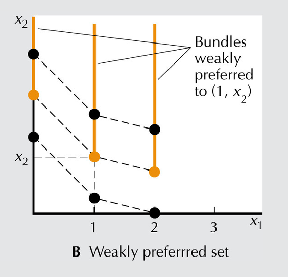
Discrete goods
When a good only comes in whole units (a discrete good), the indifference "curve" is really a set of separate points, one at each whole-number amount. A dotted line can link the points to show the pattern, but only the points are real bundles. (This is from the textbook. It is not on the slides and McLeod did not cover it in class.)
Well-behaved preferences
The axioms aren't enough to get the nice indifference curves used for the rest of the term. Two more assumptions are needed.
Well-behaved preferences
Preferences are well-behaved if they are both monotonic and convex.
- NOTE: The preferences for two goods that are perfect complements are both monotonic and convex. (Only in a weak sense. Under the strict definition of monotonicity below, they fail:
has more of good 1 than but is not better. They are convex, but not strictly convex. McLeod did not cover this in class.)
McLeod said these two assumptions give "nice well-behaved indifference curves so that we can play around with for the rest of the term." Expect them to be assumed in almost every later problem.
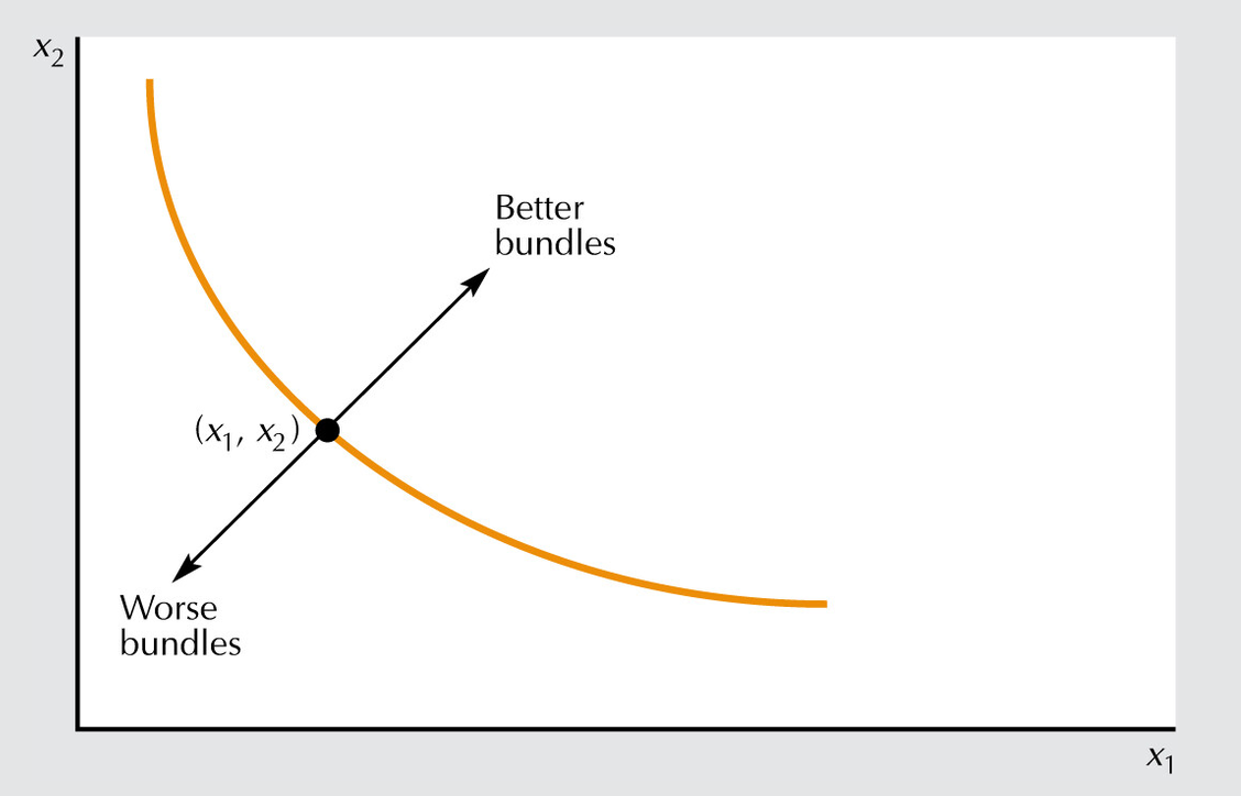
Monotonicity
More of any commodity is always preferred. This means there is no satiation, and both commodities are goods rather than 'bads' or neutrals. This then implies that indifference curves have a negative slope.
Why: It's the fancy way of saying we work in the region below and to the left of the satiation point, where the consumer wants more of both. We're basically worrying about consumption of goods before satiation hits (not that its inexistent altogether)
- If
and are bundles of goods where has at least as much of both goods and more of one, then - NOTE: THIS ALSO IMPLIES THAT INDIFFERENCE CURVE MUST HAVE A NEGATIVE SLOPE
Convexity
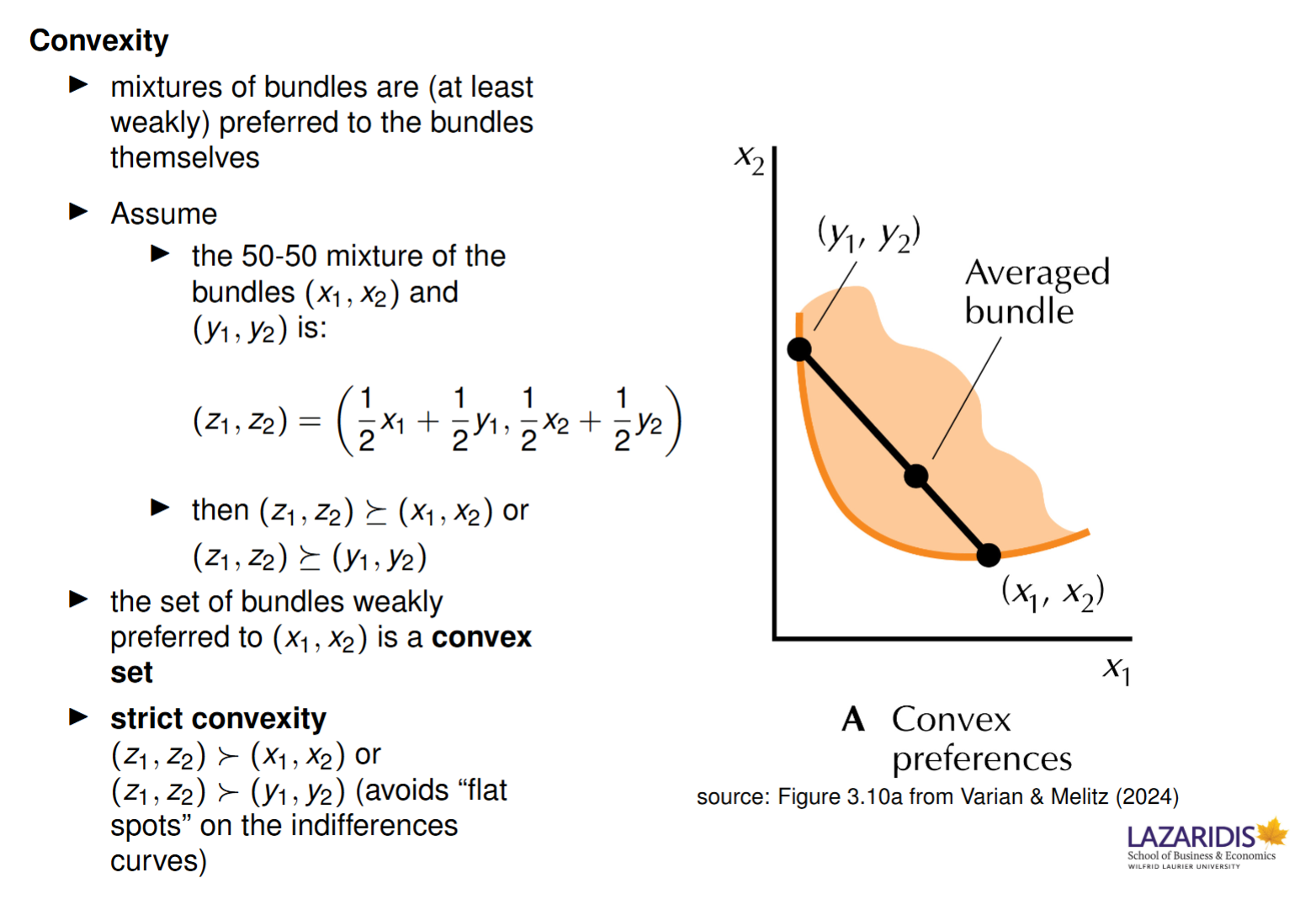
Averages are at least as good as extremes. Take two bundles X and Y that the consumer is indifferent between, and mix half of each into a new bundle Z. Under convexity, Z is weakly preferred to X and to Y. Graphically, the straight line joining X and Y sits in the weakly preferred set.
- Strict convexity: the mixture is strictly preferred. It lands in the shaded strictly preferred area, and the curve bows toward the origin with no "flat spots".
- Weak convexity: straight-line indifference curves, like perfect substitutes, are also allowed. The mixture lands right on the curve, so the consumer is indifferent to it.
Why: Convexity rules out indifference curves with "holes" in the preferred set. It keeps the curves either bowed toward the origin or straight.
where
A consumer is indifferent between
-- average the good 1 amounts -- average the good 2 amounts -- the mixed bundle, halfway along the line from X to Y - With perfect substitutes:
, and -- all three bundles have the same total, so Z is on the same line (weak convexity)
Answer: Under convexity,
Non-convex and concave preferences
These are the cases convexity rules out:
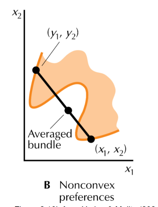
- Non-convex preferences: the curve has a dip, so the average bundle can fall outside the preferred set. That leaves a "hole" in the preferred set, which McLeod called "wonky preferences". Usually very weird-shaped graphs.
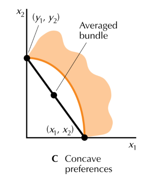
- Concave preferences: the extreme case. The curves bow away from the origin, so the whole line between X and Y lies below the curve. The consumer likes a mixture less than all of one or all of the other: they "don't like averages".
The marginal rate of substitution
This topic looks at how a consumer moves from one bundle to another while staying on the same indifference curve.
Marginal rate of substitution
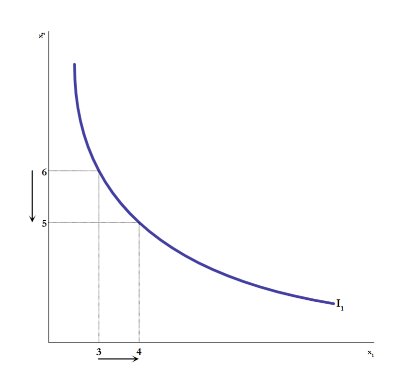
The marginal rate of substitution (MRS) is the rate at which the consumer is just willing to give up one good to get more of the other while staying on the same indifference curve. It is the slope of the indifference curve.
Why: The slope has an economic meaning: it shows how much of good 2 the consumer will give up to get one more unit of good 1.
- Slope (MRS)
- the rate at which the consumer is just willing to substitute a little more consumption of good 2 for a little less consumption of good 1 (this is the opposite way of the graph above) - In the slide example, where the MRS is about
, we interpret this as the consumer being willing to give up one unit of to get one more unit of . In general, the MRS is how many units of they give up per extra unit of . Also, the MRS will always increase (become less negative) as increases. The slides say this is the case if and only if we have preferences that are strictly convex.
where
The consumer moves along
-- gain one unit of good 1 -- give up one unit of good 2 -- the approximate slope between the two points
Answer: The MRS is about
How the MRS changes along a curve
On a curved indifference curve, the slope is different at each point (McLeod said you should remember this from MA 129). So the consumer's willingness to trade depends on how much of each good they already have. With strictly convex preferences, the MRS increases as
Why: When you have lots of good 2 and little good 1, you'll give up a lot of good 2 for one more unit of good 1. Once you already have lots of good 1, you'll give up very little. The concave case reads oddly: the consumer gives up a lot of the good they're short on. That fits with concave consumers rushing toward "all of one" good.
On a convex curve, the steep upper-left part has
-- at the steep point, the consumer gives up 5 units of good 2 -- at the flat point, the consumer gives up only half a unit of good 2
Answer: With a lot of good 2, one more unit of good 1 is worth 5 units of good 2. With a lot of good 1, it is worth only half a unit.
On a concave curve, the flat upper-left part has
-- at the upper-left point, where good 2 is plentiful, the consumer gives up only half a unit of good 2 -- at the lower-right point, where good 2 is scarce, the consumer gives up 5 units of good 2
Answer: The MRS becomes more negative as
The MRS for special shapes
The MRS describes the shape of an indifference curve:
- Perfect substitutes:
everywhere, a constant. The consumer always trades one for one. - Neutrals: with the neutral on the vertical axis (as on the slides), the MRS is infinite everywhere, because the curves are vertical.
- Perfect complements: the MRS is either 0 (the flat arm) or infinite (the vertical arm), with nothing in between. Strictly speaking, the slope is undefined at the corner.
- More Behaviours of the MRS
- MRS
when we are dealing with perfect substitution. - MRS
when we're dealing with a neutral good - MRS
or WHEN we're dealing with perfect complements
- MRS
Diminishing marginal rate of substitution
Monotonicity means indifference curves slope downward, so getting more of one good always means giving up some of the other. Convexity means the MRS falls in absolute value as
Exam checklist
- #A good with a negative price: the slope is
, not . A negative price gives an upward-sloping line. - #Transitivity: "the most important of the three" axioms.
- #Indifference curves cannot cross: know the proof by contradiction using transitivity.
- #Well-behaved preferences: monotonic plus convex, used for the rest of the term.
Admin & deadlines
- There was no tutorial on Friday, September 18. Tutorials start Friday, September 25. From the syllabus: tutorial iClicker marks (5%, best 8 of 10) start in Week 3, so they count from that first tutorial.
- McLeod cancelled the Thursday, September 17 office hours (1:30 to 2:30pm) and said an announcement would go up on MyLearningSpace. To meet another time, email McLeod at [email protected]. The syllabus says to put "EC270" in the subject line, or you may not get a reply.
- Chapter 3 is finished and the class is on schedule. Section B stopped 10 minutes early to stay level with Section A. The next lecture is Tuesday, September 22, on Chapter 4: Utility.
- From the syllabus, not mentioned in class: Assignment 1 covers Chapters 2 and 3. It is due on Smartwork5 by 11:59pm on Sunday, September 27. Late work loses 25% per day, and only your best 5 of the 6 assignments count (2% each).
- From the syllabus, not mentioned in class: the midterm is Friday, October 30, 5:00 to 7:00pm. If you will miss it for religious observance, an academic conflict or varsity athletics, you may be able to write it at another time, but only if you give written notice by Thursday, September 24.
Transcribed automatically from the lecture recording. Slides used: EC 270 - Ch. 03 - Preferences (slides).pdf. Course info used: EC 270 - Math Appendix (slides).pdf, EC 270 - Rules of Derivatives.pdf, EC 270 - Syllabus - Fall 2026.pdf. Audio archived at /mnt/porsche/configs/lectures/archive/2026-09/EC 270 - 2026-09-17 - Lecture 03.opus.