Chapter 14 - Notes
14.1 - Macroeconomic Investment
Key Definition
- Investment (macro definition): spending on new capital assets that increase the economy's productive capacity
- This is NOT what most people mean by "investing" — buying stocks, gold, or land is NOT macroeconomic investment because you're just buying existing assets, not creating new productive capacity
- Don't confuse saving and investment:
- Saving = money left over after spending
- Investment = actual spending on new capital
- They're related: your bank can lend your savings to a business that uses it to build a factory (that's investment)
Capital Stock and Depreciation
- Capital stock: the total quantity of capital at a point in time
- Investment adds to the capital stock (it's a flow of new spending)
- Depreciation subtracts from it (wear and tear, obsolescence, aging, damage)
- This year's capital stock = last year's capital stock − depreciation + new investment
- Capital stock rises when investment > depreciation, falls when depreciation > investment
Three Types of Investment
1. Business Investment (largest category)
- Equipment: computers, machinery, company cars
- Structures: offices, stores, factories, remodelling
- Intellectual property: software, R&D, TV/movie/music production
- All increase the productive capacity of the economy
2. Inventories (smallest category)
- Raw materials, work-in-progress, unsold goods (e.g., cars at a dealership)
- Change in inventories is tiny as a share of total investment BUT very volatile
- Unsold goods build up fast when sales are weak → big quarter-to-quarter swings
3. Housing Investment
- Building new houses/apartments + improvements to existing housing
- Buying an existing home does NOT count — just transfers ownership, no new productive capacity
- Renovating a home DOES count — increases productive capacity
- New housing counts because it increases the economy's capacity to generate rent (even if you live in it yourself — opportunity cost principle)
Why Investment Matters So Much
- Investment is only ~18% of GDP (~$12,900 per person/year) but economists watch it closely because:
1. Investment drives the business cycle
- Investment fluctuates WAY more than GDP — GDP might drop 2% in a recession but investment can drop 20%+
- Why so volatile?
- Managers can easily delay or cancel expansion plans
- Investment is forward-looking → extremely sensitive to expectations about the future economy
- Often requires loans → sensitive to financial sector conditions
- "Once you figure out what drives investment, you've figured out much of what drives the business cycle"
2. Investment changes quickly but capital stock changes slowly
- Capital stock is the accumulation of years of past investment → doesn't move much year to year
- Provides a stable link between last year's economy and this year's
3. Investment drives long-term prosperity
- More capital per worker → more productive workers → more output per worker
- Countries with more capital per worker are typically more prosperous
- Human capital (education) also drives productivity but isn't counted in macro investment — if it were, the role of investment would be even bigger
14.2 - Tools to Analyze Investments
Core idea: Investment decisions involve costs today and benefits in the future. To compare them, you need tools to convert money between different points in time.
Tool 1: Compounding
- Compounding tells you what money today will grow into in the future
- Compound interest: you earn interest not just on your initial deposit, but also on previously earned interest — your wealth snowballs
- Each year, your balance is multiplied by (1 + r), where r is the interest rate
Compounding formula:
- Future Value = Present Value × (1 + r)^t
- r = interest rate (as a decimal, e.g., 6% = 0.06)
- t = number of years
- e.g., $4 million at 6% for 30 years = $4M × (1.06)^30 = ~$23 million
- The longer you leave money to compound, the more dramatically it grows — this is why financial advisors say start saving early
Tool 2: Discounting
- Discounting is the reverse of compounding — it converts future money into what it's worth today
- Present value: the amount you'd need to invest today to produce an equivalent amount in the future
- The logic: money in the future is worth less than money today because of the opportunity cost of not being able to earn compound interest on it in the meantime
Discounting formula:
- Present Value = Future Value / (1 + r)^t $$\text{Present Value} = \frac{\text{Future Value}}{(1 + r)^t}$$
- Same equation as compounding, just rearranged
- e.g., what's $1 million in 14 years worth today at 6%? → $1,000,000 / (1.06)^14 = $442,301
- Meaning: you could create that $1 million by just putting $442,301 in the bank today at 6% for 14 years
The two formulas are just inverses of each other:
- Compounding: present → future (multiply by (1 + r)^t)
- Discounting: future → present (divide by (1 + r)^t)
Real vs Nominal Interest Rates in These Formulas
- Use the nominal interest rate if you want to know how many actual dollars you'll have (nominal future value)
- Use the real interest rate (nominal rate − inflation) if you want to know your actual purchasing power (real future value)
- This makes a huge difference over time:
- $1,000 at 10% nominal for 90 years = ~$5.3 million (nominal)
- $1,000 at 6.9% real for 90 years = ~$405,000 (real purchasing power)
- Same money, but inflation of 3.1%/year makes the real value way smaller
14.3 - Making Investment Decisions
Core Rule
- Rational Rule for Investors: invest if the present value of future revenues > the up-front cost (C)
- This is just the cost-benefit principle applied to investments, using present values to make costs and benefits comparable
How to Evaluate an Investment (Step by Step)
Step 1: Determine the up-front cost
- If the cost is paid today, the present value of the cost is just the cost itself
- e.g., a wind turbine costs $4 million today → PV of cost = $4 million
Step 2: Forecast future revenues, accounting for depreciation
- Depreciation rate (d): the proportion of an investment's remaining productive capacity lost each year
- Revenue declines each year by d%
- e.g., first year revenue = $600,000, depreciation rate = 4%
- Second year = $600,000 × (1 − 0.04) = $576,000
- Third year = $576,000 × (1 − 0.04) = $552,960, and so on
Step 3: Discount each year's revenue back to present value
- Apply the discounting formula to each year's revenue using the real interest rate
- Add up all the present values to get the total present value of benefits
Shortcut — The Valuation Formula:
- PV of stream of payments = Next year's revenue / (r + d)
- r = real interest rate, d = depreciation rate
- e.g., $600,000 / (0.06 + 0.04) = $600,000 / 0.10 = $6 million
- Works when revenue starts next year and declines at a constant rate over a long time
- This gives the same answer as adding up every single year's discounted revenue — just way faster
Step 4: Compare PV of benefits to PV of costs
- If PV of benefits > cost → invest (it's profitable)
- e.g., $6 million in benefits > $4 million cost → invest, adds $2 million in value
Alternative Perspective: The User Cost of Capital
Instead of evaluating the whole lifetime of an investment, you can ask: "should I buy this machine for just one more year?"
User cost of capital = the extra cost of using one more machine for one year
- Two components:
- Depreciation cost = d × C (the machine loses value)
- Foregone interest = r × C (opportunity cost of tying up your money)
- User cost = (r + d) × C
- e.g., (0.06 + 0.04) × $4,000,000 = $400,000
Decision rule: invest if next year's revenue > user cost of capital
- e.g., $600,000 revenue > $400,000 user cost → invest
Both approaches give the same answer:
- Lifetime approach: PV of all future revenues > up-front cost?
- Annual approach: next year's revenue > user cost of capital?
- They're mathematically equivalent — use whichever is easier for the problem
Education as an Investment (important application)
- Same framework: up-front cost (tuition + foregone wages) vs. PV of higher lifetime earnings
- Bachelor's degree holders earn ~$20,000/year more than high school grads
- Using the valuation formula with d = 2%, r = 3%: PV = $20,000 / (0.03 + 0.02) = $400,000
- Cost of university is almost certainly less than $400,000 → very profitable investment
14.4 - The Macroeconomics of Investment
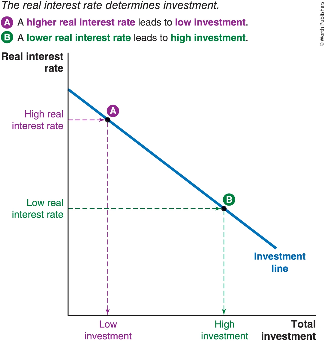
The Real Interest Rate and Investment
- The real interest rate is the central driver of investment decisions
- Why? The opportunity cost principle — the alternative to investing in a machine is leaving money in the bank earning interest
- Higher real interest rate → less investment
- Higher interest rate raises the user cost of capital
- Higher interest rate lowers the present value of future revenues (because you're discounting more heavily)
- Fewer projects pass the Rational Rule for Investors test
- Lower real interest rate → more investment
- The investment line is downward-sloping: as real interest rate falls, quantity of investment rises
- A change in the real interest rate = movement ALONG the investment line (not a shift)
Example of how interest rate matters:
- Wind turbine: $600,000 first year revenue, d = 4%, cost = $4M
- At r = 6%: PV = $600K / (0.06 + 0.04) = $6M > $4M → invest
- At r = 8%: PV = $600K / (0.08 + 0.04) = $5M > $4M → still invest
- At r = 12%: PV = $600K / (0.12 + 0.04) = $3.75M < $4M → do NOT invest
Key Distinction: Movement Along vs Shift of the Investment Line
- Change in real interest rate = movement along the investment line
- Change in other factors = shifts the investment line left or right
- Rightward shift = more investment at any given interest rate (conditions improved)
- Leftward shift = less investment at any given interest rate (conditions worsened)
Investment Shifters
1. Technological Advances
- New tech makes capital more productive → more revenue per unit of capital → more projects are profitable
- Tech that reduces the depreciation rate also helps — lower d means higher PV of future revenues (remember the valuation formula: revenue / (r + d), so lower d = higher PV)
- Shifts investment line right
2. Expectations
- Investment is forward-looking — driven by expectations about FUTURE revenues, not past revenues
- Optimism about future economy → managers forecast higher revenues → more investment → shifts right
- Pessimism → lower revenue forecasts → fewer profitable projects → shifts left
- Sometimes called "animal spirits" — the mood/confidence of managers can drive investment swings
3. Corporate Taxes
- Higher corporate taxes → companies keep less of their profits → effectively reduces revenue from investments → shifts left
- Tax breaks/incentives (e.g., for wind farms) → increases after-tax revenue → shifts right
4. Lending Standards and Cash Reserves
- Investment requires up-front cash, but revenues come later → creates a financing problem
- Most companies borrow from banks to fund investment
- If lending standards are strict (banks don't want to lend for risky projects) → less investment even if projects are profitable → shifts left
- Looser lending standards or companies having more cash reserves → more investment → shifts right
Summary Table
| Factor | Investment shifts RIGHT when... | Investment shifts LEFT when... |
|---|---|---|
| Technological advances | Better tech / lower depreciation | — |
| Expectations | Optimistic | Pessimistic |
| Corporate taxes | Lower taxes / tax breaks | Higher taxes |
| Lending standards / cash | Easier lending / more cash | Tighter lending / less cash |
And remember: real interest rate changes are movements ALONG the curve, not shifts.
14.5 - The Market for Loanable Funds
Supply is three buckets: Canadian households saving, the Canadian government saving (if it runs a surplus), and foreigners lending money to Canada
Key Setup
- Loanable funds market: the market where savers (suppliers) lend funds to investors (demanders) who want to borrow to fund capital investments
- The price in this market = the real interest rate
- The financial sector (banks, bond market, stock market) is the marketplace connecting savers and investors
- This market determines the long-run (neutral) real interest rate
- Neutral real interest rate: the interest rate when the economy is operating at its potential — not above or below capacity
- Short-run interest rate movements are driven by Bank of Canada policy (Chapter 22); long-run rate is driven by supply and demand of loanable funds
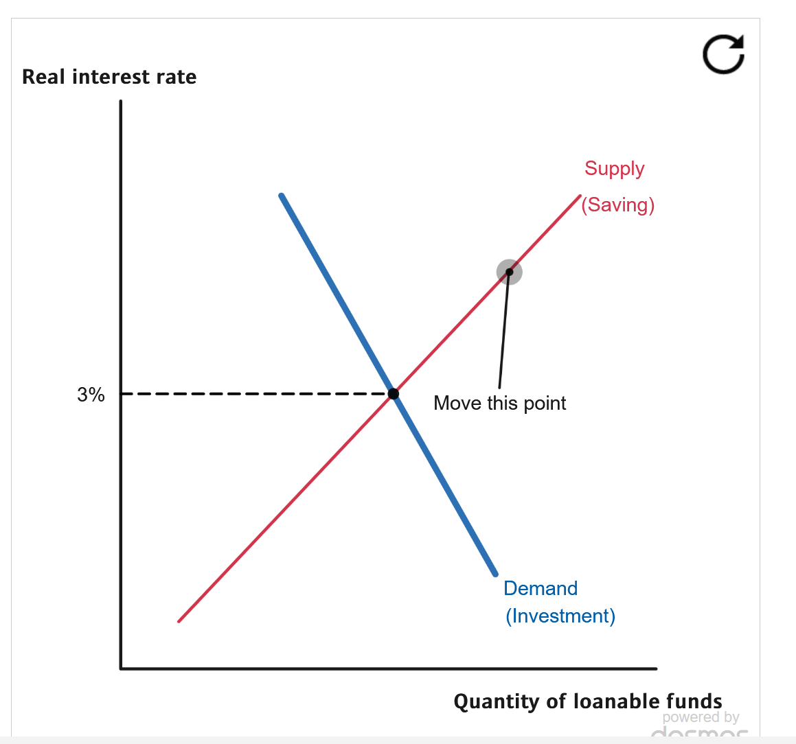
Supply and Demand Curves
- Supply (from savers) is upward-sloping: higher real interest rate → greater reward for saving → more funds supplied
- Demand (from investors) is downward-sloping: higher real interest rate → fewer profitable investment projects → less funds demanded
- Equilibrium where they cross determines the neutral real interest rate AND the quantity of saving/investment
Shifts in Supply of Loanable Funds (Three Shifters)
1. Changes in Personal Saving Rates
- Anything that makes people save more → supply shifts right → lower real interest rate
- Anything that makes people save less → supply shifts left → higher real interest rate
- e.g., government tax breaks for retirement savings encourage saving → supply shifts right
2. Government Budget Surplus or Deficit
- Budget surplus (revenue > spending) = government saving → adds to supply → shifts right
- Budget deficit (spending > revenue) = government dissaving → government must borrow → reduces supply → shifts left → higher interest rate
- Crowding out: when government borrowing pushes up real interest rates, which crowds out private investment that would have been funded at the lower rate
- Exception: if Canada borrows internationally, domestic investment may not be crowded out (but affects exchange rates and trade)
3. Global Shocks / Foreign Saving
- Foreign saving = money flowing into Canada from foreign lenders (net financial inflows)
- If foreign saving increases (e.g., Asian savings glut in early 2000s) → supply shifts right → lower real interest rate
- If foreign saving decreases → supply shifts left → higher real interest rate
Shifts in Demand for Loanable Funds (Four Shifters)
These are the same four investment shifters from 14.4 — since investment = demand for funds:
- Technological advances → more productive capital → demand shifts right → higher interest rate
- Optimistic expectations → higher expected revenues → demand shifts right → higher interest rate
- Corporate tax cuts → businesses keep more revenue → demand shifts right → higher interest rate
- Easier lending standards / more cash reserves → demand shifts right → higher interest rate
Opposite direction for each → demand shifts left → lower interest rate
How to Analyze Any Scenario (3-Step Recipe)
- Does this affect saving (supply) or investment (demand)?
- Does the curve shift right (increase) or left (decrease)?
- What happens to the real interest rate and quantity of saving/investment?
Important Practice Scenarios from the Textbook:
- Corporate tax cut → more investment → demand right → higher r, more S&I
- Foreign "safe haven" inflows → more supply → supply right → lower r, more S&I
- Government deficit → less public saving → supply left → higher r, less S&I (crowding out)
- More parents saving for university → more private saving → supply right → lower r, more S&I
- Pessimistic profit expectations → less investment → demand left → lower r, less S&I
- Nominal interest rate rises by 2% due to 2% higher inflation → TRICK QUESTION — real interest rate unchanged → no shift in either curve → no effect
Secular Stagnation
- Several long-term trends have shifted demand for loanable funds left, pushing the neutral real interest rate very low:
- Slowing population growth → less investment needed to equip new workers
- Tech firms don't need much physical capital (e.g., WhatsApp worth as much as Sony, no factories)
- Capital equipment (especially computers) getting cheaper → businesses need fewer funds
Questions
- We observe that the long-run interest rate has increased, and the equilibrium quantity of savings and investment has fallen. Which of the following changes would have caused this?
An increase in the government budget deficit