Chapter 18 - Notes
18.1 - Aggregate Expenditure
Key Definition
- Aggregate expenditure (AE): the total amount of goods and services people want to buy across the whole economy
- AE = C + I + G + NX
- C = Consumption
- G = Government purchases
- I = Planned investment (excludes unplanned inventory buildup)
- NX = Net exports (exports − imports)
- Uses planned investment because you want to measure what people actually want to buy, not unsold stuff sitting in warehouses
The Core Idea: Output Adjusts to Meet Aggregate Expenditure
- If output > AE → unsold inventories pile up → businesses cut production
- If output < AE → businesses are selling faster than producing → they ramp up production
- Macroeconomic equilibrium: when total output (GDP) = aggregate expenditure
- Y = AE (where Y = GDP)
- In the short run, demand drives output — if people don't want to buy, businesses won't produce
The Demand-Driven Short Run vs Supply-Driven Long Run
- Long run (decade+): focus on supply side — labour, capital, technology determine potential output (grows smoothly over time)
- Short run (year-to-year fluctuations): focus on demand side — aggregate expenditure determines actual output (moves in fits and starts)
- Actual GDP can differ from potential GDP:
- Actual < potential (negative output gap): weak aggregate expenditure → production lines idle, workers unemployed — this CAN be an equilibrium because businesses won't produce what people won't buy
- Actual > potential (positive output gap): economy overheating — extra shifts, deferred maintenance, overtime — not sustainable, eventually sparks inflation
Equilibrium GDP vs Potential GDP — DON'T CONFUSE THESE
- Equilibrium GDP: the level where output = aggregate expenditure — where the economy actually comes to rest
- Potential GDP: the economy's highest sustainable level of production — determined by available inputs
- They can be different! Equilibrium GDP can be below (or above) potential GDP
- The goal is for equilibrium GDP to equal potential GDP — the "Goldilocks" outcome
Output Gap Language
- Don't say the output gap got "bigger" or "smaller" — it's confusing because of negative numbers
- Instead say more negative (economy further below potential) or more positive (economy further above potential)
- e.g., going from −2% to −3% = more negative output gap
- e.g., going from −2% to −1% = more positive output gap
18.2 - The IS Curve: Output and the Rael Interest Rate
The Real Interest Rate is the Key Price
- The real interest rate (r) represents the opportunity cost of spending — you can spend now, or save, earn interest, and buy more later
- Higher r = higher opportunity cost of spending = people spend less
- Lower r = lower opportunity cost = people spend more
- The Bank of Canada uses the interest rate as its main tool to influence the economy
How the Real Interest Rate Affects Each Component of AE
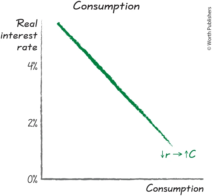
1. Lower r → Higher Consumption
- Lower opportunity cost of spending now instead of saving
- Lower cost of borrowing for big-ticket items (cars, houses)
- Exception: people who live off interest income (retirees) may consume less — but this effect is small overall
2. Lower r → Higher Investment (the MOST sensitive component)
- Lower opportunity cost of investing in equipment/structures vs putting money in the bank
- A low enough rate can make billions of dollars of investment projects worth pursuing
- Investment is the most interest-rate-sensitive component of AE
3. Lower r → Higher Government Purchases (sometimes)
- Lower interest payments on government debt → more money left in the budget for spending on roads, bridges, etc.
- But governments might use the savings to pay down debt instead, so this effect isn't guaranteed
4. Lower r → Higher Net Exports (indirect mechanism)
- Lower Canadian interest rate → international investors send money elsewhere for better returns → less demand for C$ → Canadian dollar depreciates
- Cheaper C$ → Canadian exports cheaper for foreigners → exports rise
- Cheaper C$ → imports more expensive for Canadians → imports fall
- Exports up + imports down = net exports rise
The Chain: ↓r → ↑C + ↑I + ↑G + ↑NX → ↑AE → ↑GDP → more positive output gap
The IS Curve
- IS curve: shows the relationship between the real interest rate and the output gap
- Named because it describes Investment and Spending decisions / Interest Sensitivity of output
- Think of it as a macroeconomic demand curve
- Vertical axis: real interest rate (the price/opportunity cost of spending)
- Horizontal axis: output gap (total quantity of output relative to potential)
- The IS curve is downward-sloping: lower real interest rate → more spending → higher output → more positive output gap
How to Use the IS Curve
- Pick a real interest rate on the vertical axis → read across to the IS curve → read down to find the corresponding output gap
- e.g., at r = 4%, output gap might be −5%; at r = 1%, output gap might be +2.5%
Movement Along vs Shift
- Change in the real interest rate = movement ALONG the IS curve
- Change in other factors that affect AE at a given interest rate = SHIFT of the IS curve (covered later)
Historical Example: Early 1990s Recession
- Bank of Canada raised real interest rate to over 9% to fight inflation
- Result: investment fell sharply, consumption fell, C$ appreciated (hurting net exports) → AE fell → GDP fell below potential → unemployment rose from 8% to 11.7%
- But it worked: inflation fell to ~2% and stayed there for 30 years
- Demonstrates the IS curve in action — high r → negative output gap
18.3 - The MP Curve: What Determines the Interest Rate
Two Forces Determine the Real Interest Rate
Real interest rate = Risk-free rate (set by Bank of Canada) + Risk premium (determined by financial markets)
1. The Bank of Canada Sets the Risk-Free Rate
- 8 times a year, the Governing Council meets to decide the interest rate
- This process is called monetary policy
- The Bank sets the nominal interest rate, but since it accounts for inflation, it's effectively setting the real interest rate
- e.g., nominal rate = 5%, inflation = 2% → real rate = 3%
- Specifically, the Bank targets the overnight rate — the interest rate on very short-term, nearly risk-free overnight loans
- Changes in this rate percolate through the whole economy — affecting savings rates, mortgage rates, credit card rates, business borrowing rates, etc.
2. Financial Markets Determine the Risk Premium
- Risk premium: the extra interest lenders charge to compensate for the risk of lending
- Riskier loans → higher risk premium → higher interest rate
- e.g., credit cards charge more than car loans because car loans have collateral (the car)
- Payday loans have outrageously high rates because borrowers are very risky
- The risk premium is a price — the price of bearing risk — determined by supply and demand in financial markets (mainly Bay Street / big banks)
- You can measure the risk premium using interest rate spreads: the difference between the interest rate on a loan and the risk-free rate (government bond rate) for the same duration
- Risk spreads are usually low and stable, but spike during financial crises (2007-2009, March 2020)
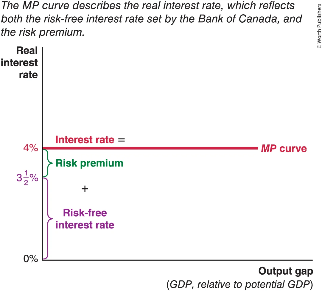
The MP Curve
- MP curve = "Monetary Policy" curve — illustrates the current real interest rate
- Drawn as a horizontal line at the current real interest rate
- e.g., if risk-free rate = 2% and risk premium = 2%, then MP curve is a horizontal line at 4%
- Horizontal because the real interest rate is the same regardless of the output gap (the Bank sets it, not the market)
- The MP curve shifts when:
- The Bank of Canada changes the risk-free rate (monetary policy change)
- Financial market conditions change the risk premium
- MP shifts up = higher real interest rate
- MP shifts down = lower real interest rate
Historical Note: IS-MP vs IS-LM
- Older textbooks use the LM curve instead of the MP curve
- The LM curve analyzed Liquidity and Money supply — more complicated because the Bank used to set the money supply instead of directly setting the interest rate
- IS-MP is simpler and reflects how modern central banks actually operate (they announce an interest rate target)
- If you see "IS-LM analysis" elsewhere, it's the same basic ideas, just an older framework
18.4 - The IS-MP Framework
Here are your notes for 18.4:
The IS-MP Framework
Putting IS and MP Together
- IS curve: shows the output gap at each possible real interest rate (downward-sloping)
- MP curve: shows the current real interest rate (horizontal line)
- Their intersection = macroeconomic equilibrium → tells you the output gap
- e.g., if MP is at r = 4% and the IS curve says that corresponds to output gap = −5%, then the economy is producing 5% below potential
Booms and Busts Explained Through the IS-MP Framework
Boom (good times):
- Optimism → consumers spend more, businesses invest more → IS curve is far to the right
- Equilibrium: output gap ≈ 0, full employment, optimism is warranted
Bust (recession):
- Pessimism → consumers cut spending, businesses cut investment → IS curve shifts LEFT
- Equilibrium: negative output gap, unemployment, economy producing below potential
- The pessimism becomes self-fulfilling — people spend less because the economy is weak, and the economy is weak because people spend less
Key insight: recessions are individually rational but collectively terrible
- Each person makes their best decision (spend less when uncertain), but those decisions add up to a bad equilibrium
- Like a concert: if everyone stands, you have to stand too (seats = unemployed) — even though everyone sitting would be better for all
- There's no guarantee the economy will fix itself — a bad equilibrium can persist unless something changes
Analyzing Monetary Policy (Bank of Canada)
- When the Bank of Canada cuts the interest rate → MP curve shifts DOWN
- → New equilibrium: higher GDP, more positive output gap
- When the Bank raises the interest rate → MP curve shifts UP
- → New equilibrium: lower GDP, more negative output gap
2008-2009 example:
- Bank cut rates from 4.25% down to 1.0% → MP shifted down dramatically → helped stabilize the economy
- But at some point, rates can't go much lower (near zero) → monetary policy runs out of ammunition
- This is why fiscal policy was also needed
Analyzing Fiscal Policy (Government Spending and Taxes)
- When the government increases spending or cuts taxes → IS curve shifts RIGHT
- → New equilibrium: higher GDP, more positive output gap, real interest rate unchanged
- When the government cuts spending or raises taxes → IS curve shifts LEFT
- → Lower GDP, more negative output gap
The Multiplier
- One person's spending = another person's income → initial spending ripples through the economy
- The multiplier measures how much total GDP changes for each extra dollar of initial spending (including all ripple effects)
- ΔGDP = ΔSpending × Multiplier
- e.g., $40 billion in government spending × multiplier of 2 = $80 billion increase in GDP
- Higher marginal propensity to consume → bigger ripple effects → larger multiplier
- The multiplier determines how far the IS curve shifts: IS shifts by ΔSpending × Multiplier
How the Multiplier Works (the ripple chain):
- Government hires construction workers to build roads (direct effect)
- Workers spend their income on cars → Ford workers earn more (first ripple)
- Ford workers buy lunch at Subway → Subway hires more staff (second ripple)
- Subway staff buy clothes → clothing store earns more (third ripple)
- And so on... each round gets smaller but they all add up
Summary: What Shifts What
| Policy action | What shifts | Direction | Effect on output gap |
|---|---|---|---|
| Bank of Canada cuts rates | MP curve | Down | More positive |
| Bank of Canada raises rates | MP curve | Up | More negative |
| Government increases spending | IS curve | Right | More positive |
| Government cuts taxes | IS curve | Right | More positive |
| Government cuts spending | IS curve | Left | More negative |
| Government raises taxes | IS curve | Left | More negative |
| Wave of optimism | IS curve | Right | More positive |
| Wave of pessimism | IS curve | Left | More negative |
| Decrease in Tax Rate | IS curve | Right | More positive |
18.5 - Macroeconomic Shocks
The Big Rule: Spending shocks shift IS, Financial shocks shift MP
Spending Shocks → Shift the IS Curve
1. Consumption — increases if people feel more prosperous
- ↑ Wealth (stock market boom, rising house prices)
- ↑ Consumer confidence (optimism about future income)
- ↑ Government assistance (e.g., more EI payments)
- ↓ Taxes (more disposable income)
- ↓ Inequality (redistributing to low-income people who spend more of their income)
2. Investment — increases if it's profitable to expand
- ↑ GDP growth (expanding economy → need more production capacity)
- ↑ Business confidence (optimism about long-term profitability)
- ↑ Investment tax credits (lower after-tax cost of new equipment)
- ↓ Corporate taxes (higher after-tax profits)
- ↑ Easier lending standards / more cash reserves
- ↓ Uncertainty (managers restart shelved projects when outlook clears)
3. Government Purchases — increases with expansionary fiscal policy
- Spending bills (highways, military, infrastructure)
- Automatic stabilizers — programs that automatically increase spending when economy is weak
- Transfer payments (EI, Old Age Security) do NOT directly shift IS — they transfer money, don't buy goods/services
- But they can indirectly boost consumption if recipients spend the money
4. Net Exports — increase due to global factors
- ↑ Global GDP growth (foreigners have more money → buy more Canadian goods)
- ↓ Canadian dollar (our exports cheaper, imports more expensive)
- ↓ Trade barriers in foreign markets (easier to sell abroad)
- ↑ Trade barriers protecting Canadian market (fewer imports)
- Trade agreements and trade wars affect both imports AND exports → net effect on NX is unclear
Remember: reverse any of these arrows and the IS curve shifts LEFT instead of right
Financial Shocks → Shift the MP Curve
1. Changes in Monetary Policy (Bank of Canada)
- ↑ Risk-free rate → MP shifts UP
- ↓ Risk-free rate → MP shifts DOWN
- Signaling expected future rate increases can also shift MP UP (because long-term rates partly reflect expectations of future short-term rates)
- Important: if inflation rises 1% and the Bank raises the nominal rate by 1%, the real rate is unchanged → MP doesn't shift
2. Changes in the Risk Premium (Financial Markets)
- ↑ Default risk (higher chance borrowers won't repay) → MP shifts UP
- ↑ Liquidity risk (banks can't easily sell loans to get cash) → MP shifts UP
- ↑ Interest rate risk (uncertainty about future rates/inflation for long-term loans) → MP shifts UP
- ↑ Risk aversion (lenders become more reluctant to take on risk) → MP shifts UP
- Reverse any of these → MP shifts DOWN
Three-Step Recipe for Any Scenario
- Is this a spending shock (IS) or financial shock (MP)?
- Which direction does the curve shift?
- What happens to GDP/output gap and the real interest rate in the new equilibrium?
Key Pattern to Remember:
- IS shifts → GDP changes but real interest rate stays the same
- MP shifts → GDP changes AND real interest rate changes
Practice Scenarios from the Textbook:
- Government cuts military spending → IS left → lower GDP, unchanged r
- Consumer confidence booms → IS right → higher GDP, unchanged r
- Risk premium rises due to uncertainty → MP up → lower GDP, higher r
- China puts tariff on Canadian exports → IS left → lower GDP, unchanged r
- Bank of Canada cuts rate → MP down → higher GDP, lower r
- Government incentives for EV factories → IS right → higher GDP, unchanged r
- European growth picks up → IS right → higher GDP, unchanged r
- Political uncertainty freezes investment → IS left → lower GDP, unchanged r
- Bank of Canada reduces risk premium → MP down → higher GDP, lower r
- Stock market crash → IS left (wealth down → consumption down) → lower GDP, unchanged r
- Bank of Canada raises rates → MP up → lower GDP, higher r
- Canadian dollar appreciates → IS left (exports more expensive) → lower GDP, unchanged r
Questions
- All else equal, an increase in the real interest rate in Canada will cause a ________________ and an ___________ in net exports.
Appreciation, decrease